Observation bias and sub-group differences can easily produce statistical paradoxes in any data science application. Ignoring these elements can therefore completely undermine the conclusions of our analysis.

It is indeed not unusual to observe surprising phenomena such as sub-groups trends that are completely reverted in the aggregated data. In this article we look at the 3 most common kinds of statistical paradoxes encountered in Data Science.

1. Berkson's Paradox

A first striking example is the observed negative association between COVID-19 severity and smoking cigarettes (see e.g. the European Commission review by Wenzel 2020). Smoking cigarettes is a well-known risk factor for respiratory diseases, so how do we explain this contradiction?

The work of Griffith 2020 recently published on Nature suggests that this can be a case of Collider Bias, also called Berkson's Paradox. To understand this paradox, let us consider the following graphical model, where we include a third random variable: "being hospitalized".

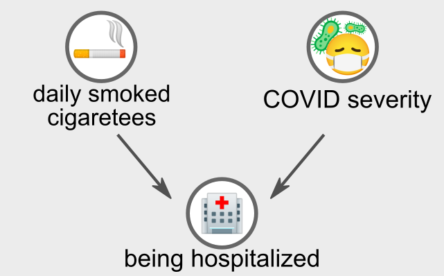
This third variable "being hospitalized" is a collider of the first two. This means that both smoking cigarettes and having severe COVID-19 increase chances of being ill in a hospital. Berkson's Paradox precisely arises when we condition on a collider, i.e. when we only observe data from hospitalized people rather than considering the whole population.

Let's consider the following example dataset. In the left figure we have observations from the whole population, while on the right figure we only consider a subset of hospitalized people (i.e. we condition on the collider variable).

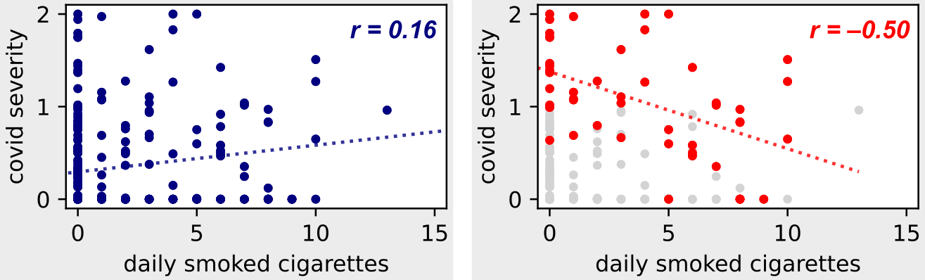
In the left figure we can observe the positive correlation between COVID-19 severity and smoking cigarettes that we expected as we know that smoking is a risk factor for respiratory diseases.

But in the right figure, where we only consider hospital patients, we see the opposite trend! To understand this, consider the following points.

1. Having high severity of COVID-19 increases chances of being hospitalized. In particular, if severity > 1 hospitalization is required.
2. Smoking several cigarettes a day is a major risk factor for a variety of diseases (heart attacks, cancer, diabetes), which increase the chances of being hospitalized for some reason.
3. Hence, if a hospital patient has lower COVID-19 severity, they have higher chances of smoking cigarettes! Indeed, they must have some disease different from COVID-19 (e.g. heart attacks, cancer, diabetes) to justify their hospitalization, and this disease may very well be caused by their smoking cigarettes.

This example is very similar to the original work of Berkson 1946, where the author noticed a negative correlation between cholecystitis and diabetes in hospital patients, despite diabetes being a risk factor for cholecystitis.

2. Latent Variables

The presence of a latent variable may also produce an apparently inverted correlation between two variables. While Berkson's Paradox arises because of the conditioning on a collider variable (which should therefore be avoided), this other kind of paradox can be fixed by conditioning on the latent variable.

Let's consider, for instance, the relation between number of firefighter deployed to extinguish a fire and the number people that are injured in the fire. We would expect that having more firefighters would improve the outcome (to some extent—see Brooks's Law), yet a positive correlation is observed in aggregated data: the more firefighters are deployed, the higher the number of injured!

To understand this paradox, let us consider the following graphical model. The key is to consider again a third random variable: "fire severity".

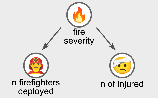
This third latent variable positively correlates with the other two. Indeed, more severe fires tend to cause more injuries, and at the same time they require more firefighters to be extinguished.

Let's consider the following example dataset. In the left figure we have aggregated observations from all kinds of fires, while on the right figure we only consider observations corresponding to three fixed degrees of fire severity (i.e. we condition our observations on the latent variable).

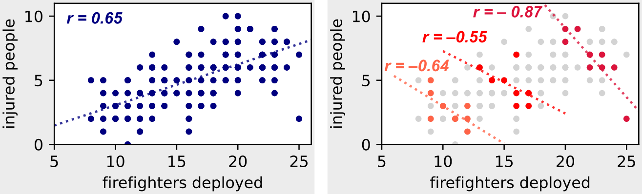
In the right figure, where we condition observations on the degrees of fire severity, we can see the negative correlation we would have expected.

• For a fire of given severity we can indeed observe that the more the firefighters deployed, the fewer the injured people.
• If the we look at fires with higher severity, we observe the same trend even though both number of firefighters deployed and number of injured people are higher.

3. Simpson's Paradox

Simpson's Paradox is a surprising phenomenon arising when a trend that is consistently observed in sub-groups, but the trend is inverted if sub-groups are merged. It is often related to the class imbalance in data sub-groups.

A notorious occurrence of this paradox is from Bickel 1975, where acceptance rates to the University of California weer analysed to find evidence of sex discrimination, and two apparently contradicting facts were revealed.

• On the one hand, in every department female applicants had higher acceptance rates than male applicants.
• On the other hands, aggregate numbers showed that female applicants had lower acceptance rates than male applicants.

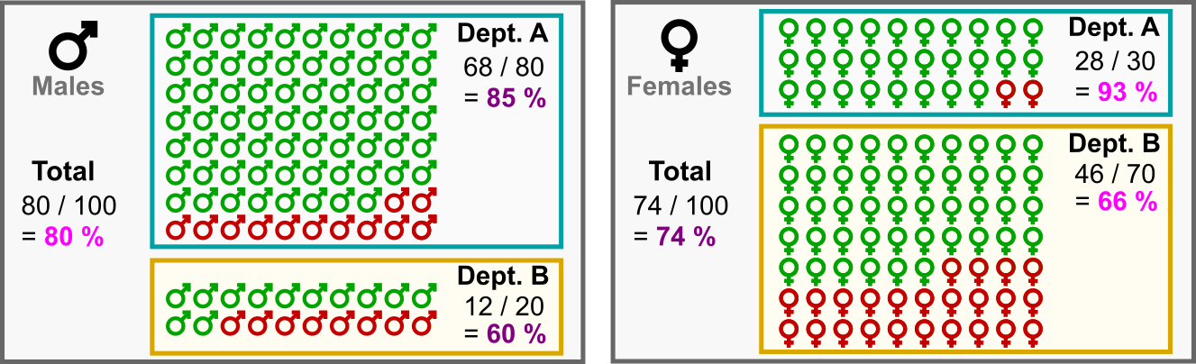
To see how this is possible, let's consider the following dataset with the two departments Dept. A and Dept. B.

• Out of 100 male applicants: 80 applied to Dept. A and 68 were accepted (85%), while 20 applied to Dept. B and 12 were accepted (60%).
• Out of 100 female applicants: 30 applied to Dept. A and 28 were accepted (93%), while 70 applied to Dept. B and 46 were accepted (66%).

The paradox is expressed by the following inequalities.

We can now understand the origin of our seemingly contradictory observations. The point is that there is a significant class imbalance in the sex of applicants in each of the two departments (Dept. A: 80–30, Dept. B: 20–70). Indeed, most female students applied to the more competitive Dept. B (which has low rates of admission), while most male students applied to the less competitive Dept. A (which has higher rates of admission). This causes the contradictory observations we had.

Conclusions

Latent variables, collider variables, and class imbalance can easily produce statistical paradoxes in many data science applications. A particular attention to these key points is therefore essential to correctly derive trends and analyse the results.