What is A/B testing?

A/B testing is one of the most popular controlled experiments used to optimize web marketing strategies. It allows decision makers to choose the best design for a website by looking at the analytics results obtained with two possible alternatives A and B.

In this article we'll see how different statistical methods can be used to make A/B testing successful. I recommend you to also have a look at this notebook where you can play with the examples discussed in this article.

To understand what A/B testing is about, let's consider two alternative designs A and B. Visitors of a website are randomly served with one of the two. Then, data about their activity is collected by web analytics. Given this data, one can apply statistical tests to determine whether one of the two designs has better efficacy.

Now, different kinds of metrics can be used to measure a website efficacy. With discrete metrics, also called binomial metrics, only the two values 0 and 1 are possible. The following are examples of popular discrete metrics.

• Click-through rate — if a user is shown an advertisement, do they click on it?
• Conversion rate — if a user is shown an advertisement, do they convert into customers?
• Bounce rate — if a user is visits a website, is the following visited page on the same website?

With continuous metrics, also called non-binomial metrics,, the metric may take continuous values that are not limited to a set two discrete states. The following are examples of popular continuous metrics.

• Average revenue per user — how much revenue does a user generate in a month?
• Average session duration — for how long does a user stay on a website in a session?
• Average order value — what is the total value of the order of a user?

We are going to see in detail how discrete and continuous metrics require different statistical test. But first, let's quickly review some fundamental concepts of statistics.

Statistical significance

With the data we collected from the activity of users of our website, we can compare the efficacy of the two designs A and B. Simply comparing mean values wouldn't be very meaningful, as we would fail to assess the statistical significance of our observations. It is indeed fundamental to determine how likely it is that the observed discrepancy between the two samples originates from chance.

In order to do that, we will use a two-sample hypothesis test. Our null hypothesis H₀ is that the two designs A and B have the same efficacy, i.e. that they produce an equivalent click-through rate, or average revenue per user, etc. The statistical significance is then measured by the p-value, i.e. the probability of observing a discrepancy between our samples at least as strong as the one that we actually observed.

Now, some care has to be applied to properly choose the alternative hypothesis H_a. This choice corresponds to the choice between one- and two- tailed tests .

A two-tailed test is preferable in our case, since we have no reason to know a priori whether the discrepancy between the results of A and B will be in favor of A or B. This means that we consider the alternative hypothesis H_a the hypothesis that A and B have different efficacy.

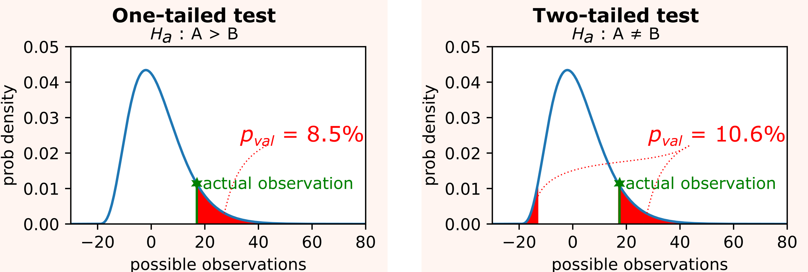
The p-value is therefore computed as the area under the the two tails of the probability density function p(x) of a chosen test statistic on all x' s.t. p(x') <= p(our observation). The computation of such p-value clearly depends on the data distribution. So we will first see how to compute it for discrete metrics, and then for continuous metrics.

Discrete metrics

Let's first consider a discrete metric such as the click-though rate. We randomly show visitors one of two possible designs of an advertisement, and we keep track of how many of them click on it.

Let's say that from we collected the following information.

• n_X = 15 visitors saw the advertisement A, and 7 of them clicked on it.
• n_Y = 19 visitors saw the advertisement B, and 15 of them clicked on it.

At a first glance, it looks like version B was more effective, but how statistically significant is this discrepancy?

Fisher's exact test

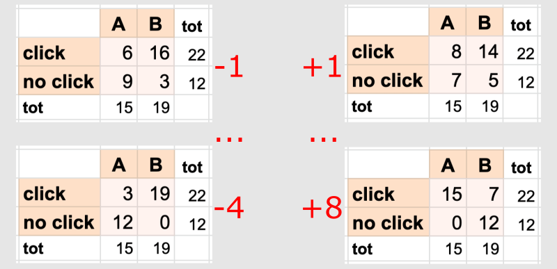
Using the 2x2 contingency table shown above we can use Fisher's exact test to compute an exact p-value and test our hypothesis. To understand how this test works, let us start by noticing that if we fix the margins of the tables (i.e. the four sums of each row and column), then only few different outcomes are possible.

Now, the key observation is that, under the null hypothesis H₀ that A and B have same efficacy, the probability of observing any of these possible outcomes is given by the hypergeometric distribution .

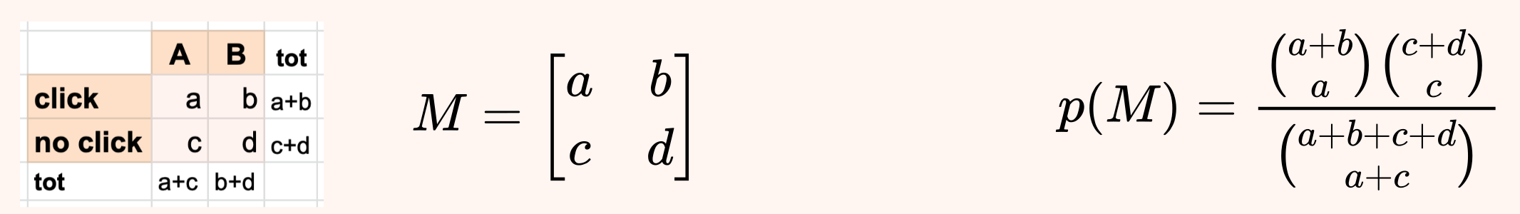
Using this formula we obtain that:

• the probability of seeing our actual observations is ~4.5%
• the probability of seeing even more unlikely observations in favor if B is ~1.0% (left tail);
• the probability of seeing observations even more unlikely observations in favor if A is ~2.0% (right tail).

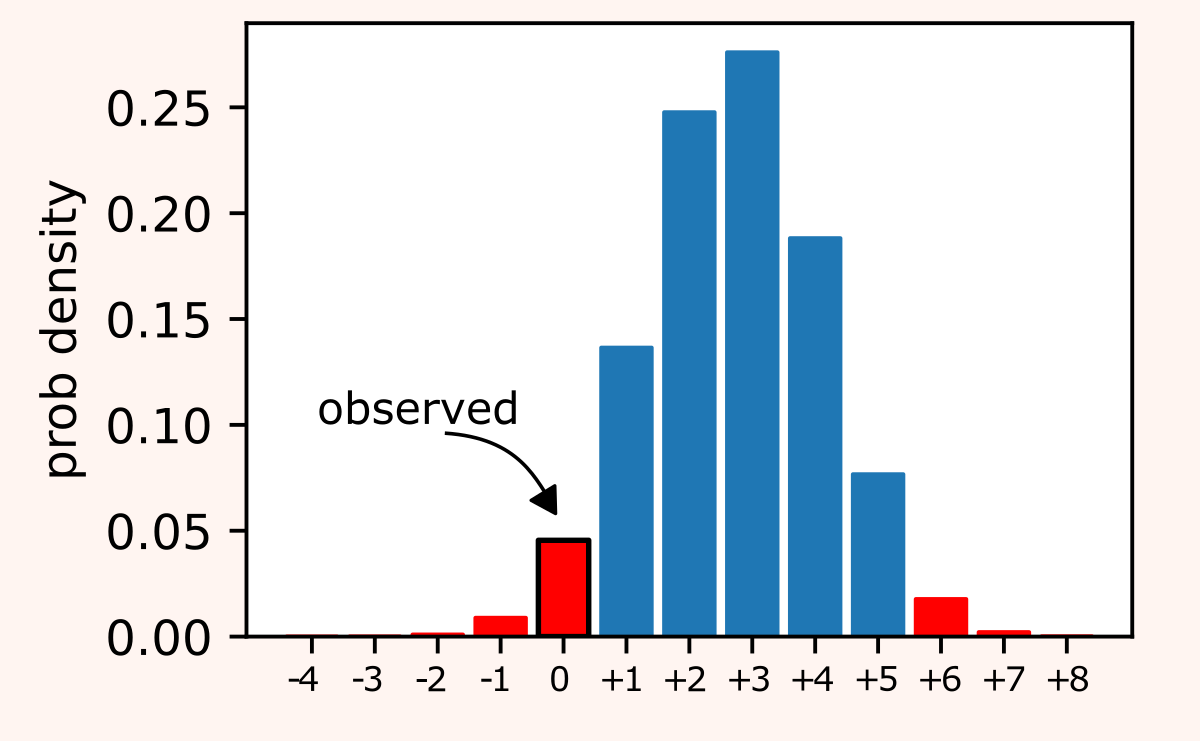
So Fisher's exact test gives p-value ≈ 7.5%.

Pearson's chi-squared test

Fisher's exact test has the important advantage of computing exact p-values. But if we have a large sample size, it may be computationally inefficient. In this case, we can use Pearson's chi-squared test to compute an approximate p-value.

Let us call O_ij the observed value of the contingency table at row i and column j. Under the null hypothesis of independence of rows and columns, i.e. assuming that A and B have same efficacy, we can easily compute corresponding expected values E_ij. Moreover, if the observations are normally distributed, then the χ² statistic follows exactly a chi-square distribution with 1 degree of freedom.

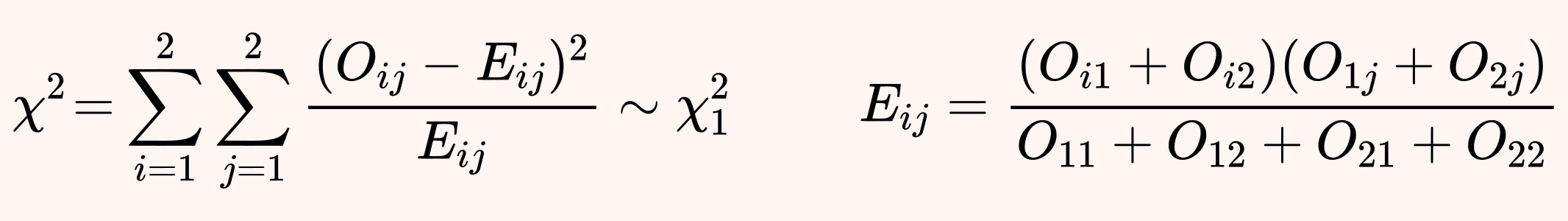
In fact, this test can also be used with non-normal observations if the sample size is large enough, thanks to the central limit theorem.

In our example, using Pearson's chi-square test we obtain χ² ≈ 3.825, which gives p-value ≈ 5.1%.

Continuous metrics

Let's now consider the case of a continuous metric such as the average revenue per user. We randomly show visitors one of two possible layouts of our website, and based on how much revenue each user generates in a month we want to determine if one of the two layouts is more efficient.

Let's consider the following case.

• n_X = 17 users saw the layout A, and then made the following purchases: 200$, 150$, 250$, 350$, 150$, 150$, 350$, 250$, 150$, 250$, 150$, 150$, 200$, 0$, 0$, 100$, 50$.
• n_X = 14 users saw the layout B, and then made the following purchases: 300$, 150$, 150$, 400$, 250$, 250$, 150$, 200$, 250$, 150$, 300$, 200$, 250$, 200$.

Again, at a first glance, it looks like version B was more effective. But how statistically significant is this discrepancy?

Z-test

The Z-test can be applied under the following assumptions.

• The observations are normally distributed (or the sample size is large).
• The sampling distributions have known variance σ_X and σ_Y.

Under the above assumptions, the Z-test exploits the fact that the following Z statistic has a standard normal distribution.

Unfortunately in most real applications the standard deviations are unknown and must be estimated, so a t-test is preferable, as we will see later. Anyway, if in our case we knew the true value of σ_X=100 and σ_X=90, then we would obtain z ≈ -1.697, which corresponds to a p-value ≈ 9%.

Student's t-test

In most cases, the variances of the sampling distributions are unknown, so that we need to estimate them. Student's t-test can then be applied under the following assumptions.

• The observations are normally distributed (or the sample size is large).
• The sampling distributions have "similar" variances σ_X ≈ σ_Y.

Under the above assumptions, Student's t-test relies on the observation that the following t statistic has a Student's t distribution.

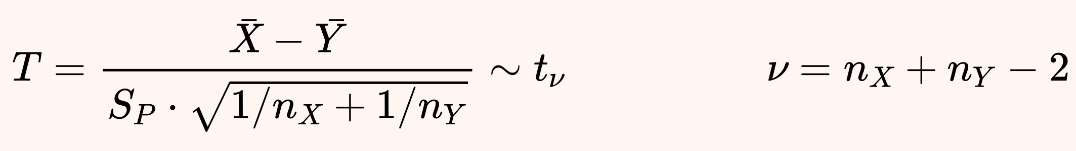
Here S_P is the pooled variance obtained from the sample variances S_X and S _Y, which are computed using the unbiased formula that applies Bessel's correction ).

In our example, using Student's t-test we obtain t ≈ -1.789 and ν = 29, which give p-value ≈ 8.4%.

Welch's t-test

In most cases Student's t test can be effectively applied with good results. However, it may rarely happen that its second assumption (similar variance of the sampling distributions) is violated. In that case, we cannot compute a pooled variance and rather than Student's t test we should use Welch's t-test.

This test operates under the same assumptions of Student's t-test but removes the requirement on the similar variances. Then, we can use a slightly different t statistic, which also has a Student's t distribution, but with a different number of degrees of freedom ν.

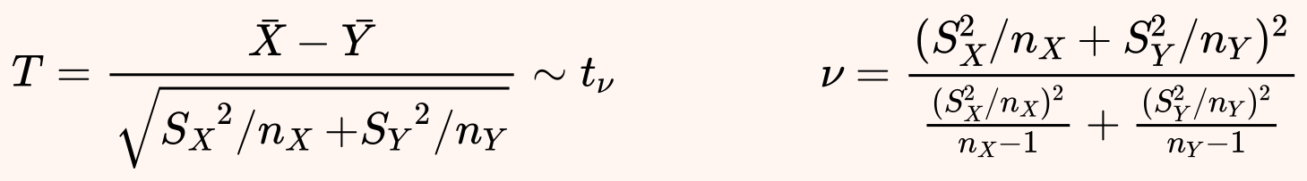
The complex formula for ν comes from Welch–Satterthwaite equation .

In our example, using Welch's t-test we obtain t ≈ -1.848 and ν ≈ 28.51, which give p-value ≈ 7.5%.

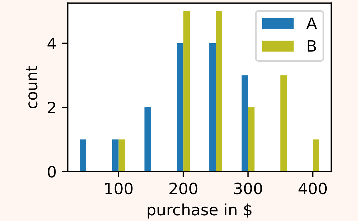
Continuous non-normal metrics

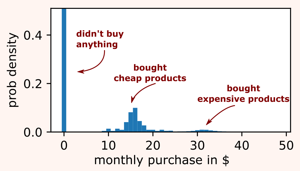
In the previous section on continuous metrics, we assumed that our observations came from normal distributions. But non-normal distributions are extremely common when dealing with per-user monthly revenues etc. There are several ways in which normality is often violated:

• zero-inflated distributions — most user don't buy anything at all, so lots of zero observations;
• multimodal distributions — a market segment tends purchases cheap products, while another segment purchases more expensive products.

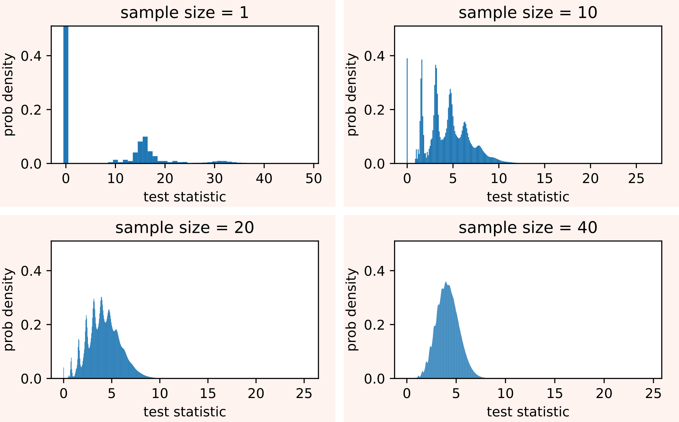
However, if we have enough samples, tests derived under normality assumptions like Z-test, Student's t-test, and Welch's t-test can still be applied for observations that signficantly deviate from normality. Indeed, thanks to the central limit theorem, the distribution of the test statistics tends to normality as the sample size increases. In the zero-inflated and multimodal example we are considering, even a sample size of 40 produces a distribution that is well approximated by a normal distribution.

But if the sample size is still too small to assume normality, we have no other choice than using a non-parametric approach such as the Mann-Whitney U test.

Mann–Whitney U test

This test makes no assumption on the nature of the sampling distributions, so it is fully nonparametric. The idea of Mann-Whitney U test is to compute the following U statistic.

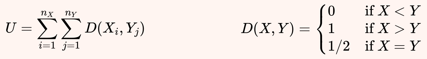
The values of this test statistic are tabulated, as the distribution can be computed under the null hypothesis that, for random samples X and Y from the two populations, the probability P(X < Y) is the same as P(X > Y).

In our example, using Mann-Whitney U test we obtain u = 76 which gives p-value ≈ 8.0%.

Conclusion

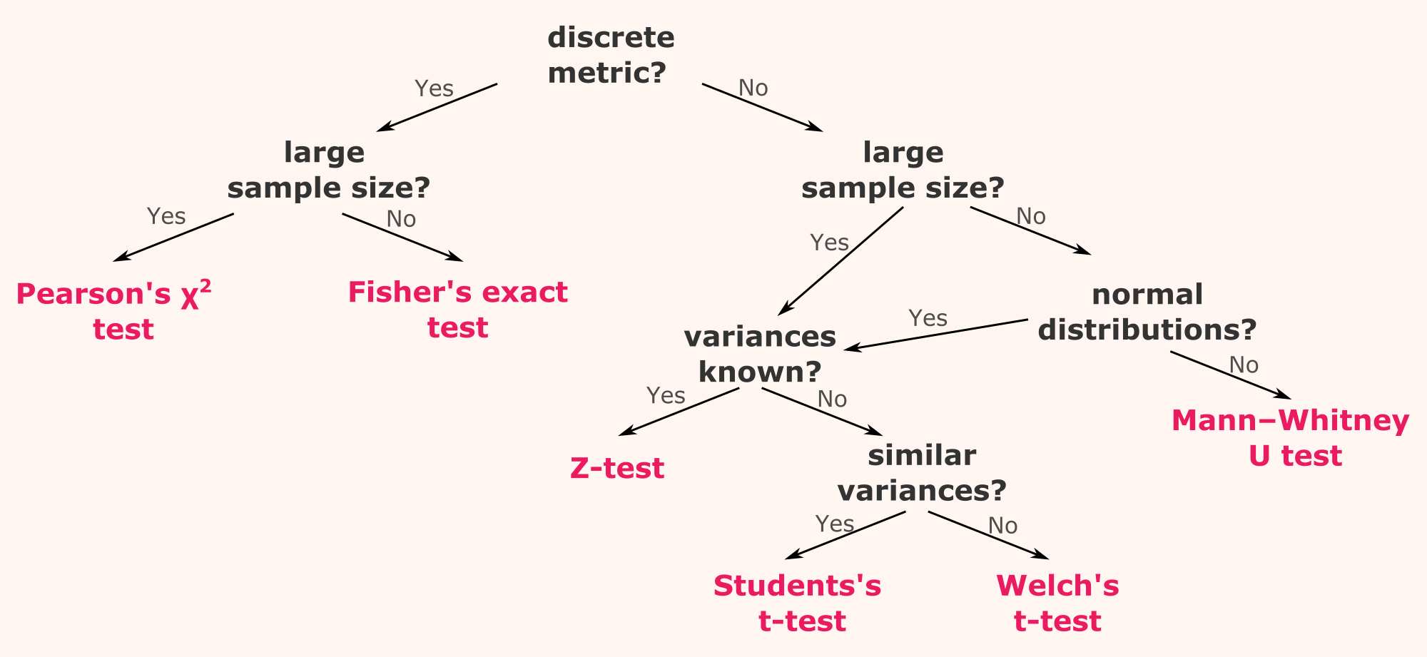
In this article we have seen that different kinds of metrics, sample size, and sampling distributions require different kinds of statistical tests for computing the the significance of A/B tests. We can summarize all these possibilities in the form of a decision tree.

If you want to know more, you can start by playing with this notebook where you can see all the examples discussed in this article.